1880-2010年全美婴儿姓名

SSA提供了一份从1880年到2010年的婴儿名字频率数据. 这也是用来做演示数据处理的好数据.

from __future__ import division
from numpy.random import randn
import numpy as np
import matplotlib.pyplot as plt
plt.rc('figure', figsize=(12, 5))
np.set_printoptions(precision=4)
import pandas as pd
# 导入全部数据
years = range(1880, 2011)

pieces = []columns = ['name', 'sex', 'births']

for year in years:
    path = 'ch02/names/yob%d.txt' % year
    frame = pd.read_csv(path, names=columns)
    frame['year'] = year
    pieces.append(frame)
names = pd.concat(pieces, ignore_index=True)
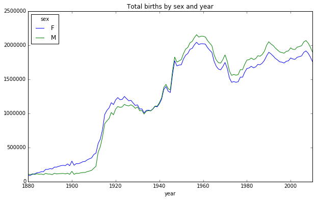
total_births = names.pivot_table('births', index='year', columns='sex', aggfunc=sum)    # 利用pivot_table对数据分组,行用年, 列用性别, 计算总数
total_births.tail()
sex     F     M
year         
2006     1896468     2050234
2007     1916888     2069242
2008     1883645     2032310
2009     1827643     1973359
2010     1759010     1898382

total_births.plot(title='Total births by sex and year')

要统计出生比例的话, 需要先添加一列prop,存放指定名字的婴儿相对于总出生数的比例. 例如prop为0.2表示100个婴儿中有2名婴儿取了当前这个名字. 先按year和sex分组.然后再加prop列到分组上

def add_prop(group):
    # 整数除法会向下圆整, 所以转换成float
    births = group.births.astype(float)

    group['prop'] = births / births.sum()
    return group
names = names.groupby(['year', 'sex']).apply(add_prop)

np.allclose(names.groupby(['year', 'sex']).prop.sum(), 1)    # 检查总数是否接近1

为更进一步分析, 需要取出一个子集: 每对sex/year组合的前1000个名字

def get_top1000(group):
    return group.sort_values(by='births', ascending=False)[:1000]
grouped = names.groupby(['year', 'sex'])
top1000 = grouped.apply(get_top1000)

另一种写法

pieces = []
for year, group in names.groupby(['year', 'sex']):
    pieces.append(group.sort_values(by='births', ascending=False)[:1000])
top1000 = pd.concat(pieces, ignore_index=True)

分析命名趋势

top1000.index = np.arange(len(top1000))    # 重建索引
boys = top1000[top1000.sex == 'M']    # 男孩前1000
girls = top1000[top1000.sex == 'F']    # 女孩前1000
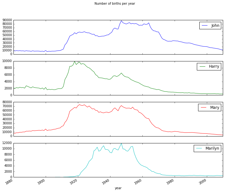
total_births = top1000.pivot_table('births', index='year', columns='name', aggfunc=sum)    # 按year和name统计的总出生数透视表
subset = total_births[['John', 'Harry', 'Mary', 'Marilyn']]    # 选取4个名字作图
subset.plot(subplots=True, figsize=(12, 10), grid=False, title="Number of births per year")    # 绘图

评估命名多样性

table = top1000.pivot_table('prop', index='year', columns='sex', aggfunc=sum)    # 按year和sex分组
table.plot(title='Sum of table1000.prop by year and sex', yticks=np.linspace(0, 1.2, 13), xticks=range(1880, 2020, 10))

途中展示了名字的多样性在逐年增长(前1000名的比例在降低). 另一种方法是计算总出生人数前50%的不同名字的数量, 这个数字不太好统计, 只考虑2010年男孩的名字:

df = boys[boys.year == 2010]    # 2010年男孩的数据
prop_cumsum = df.sort_values(by='prop', ascending=False).prop.cumsum()
prop_cumsum.values.searchsorted(0.5)
>>>116

上面的代码采用numpy中的矢量方式, 先计算prop的累计和cumsum, 然后通过searchsorted找到0.5应该被插入在哪个位置才能保证不破坏顺序. 然后拿1900年的数据做对比

df = boys[boys.year == 1900]
in1900 = df.sort_values(by='prop', ascending=False).prop.cumsum()
in1900.values.searchsorted(0.5) + 1    # 加1是因为索引从0开始
>>>25

现在对所有year/sex组合执行这个计算, 按2个字段进行groupby处理, 最后用一个函数计算各分组的值:

def get_quantile_count(group, q=0.5):
    group = group.sort_values(by='prop', ascending=False)
    return group.prop.cumsum().values.searchsorted(q) + 1
diversity = top1000.groupby(['year', 'sex']).apply(get_quantile_count)
diversity = diversity.unstack('sex')
diversity.plot(title="Number of popular names in top 50%")

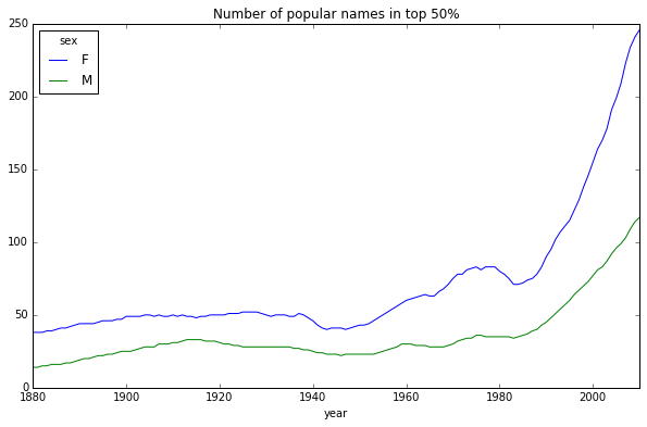图中可以看出女孩的多样性要比男孩高,而且越来越高

"最后一个字母"的变革

首先将全部出生数据在年度, 性别以及末字母上惊醒聚合

get_last_letter = lambda x: x[-1]
last_letters = names.name.map(get_last_letter)
last_letters.name = 'last_letter'
table = names.pivot_table('births', index=last_letters, columns=['sex', 'year'], aggfunc=sum)
subtable = table.reindex(columns=[1910, 1960, 2010], level='year')    # 选取代表性的3年
letter_prop = subtable / subtable.sum().astype(float)    # 计算各性别, 各末字母占总数的比例

import matplotlib.pyplot as plt

fig, axes = plt.subplots(2, 1, figsize=(10, 8))
letter_prop['M'].plot(kind='bar', rot=0, ax=axes[0], title='Male')
letter_prop['F'].plot(kind='bar', rot=0, ax=axes[1], title='Female', legend=False)

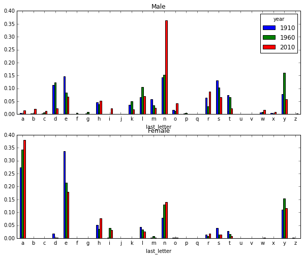图中可以看出,从60年代开始, 以字母n结尾的男孩名字出现了明显的增长.

下面选取几个字母, 按时间顺序看看变化

letter_prop = table / table.sum().astype(float)
dny_ts = letter_prop.ix[['d', 'n', 'y'], 'M'].T

dny_ts.plot()

男女孩名字转换情况

另一个现象是早起的男孩名字后期变成了女孩的名字

all_names = top1000.name.unique()
mask = np.array(['lesl' in x.lower() for x in all_names])
lesley_like = all_names[mask]
filtered = top1000[top1000.name.isin(lesley_like)]
filtered.groupby('name').births.sum()
filtered = top1000[top1000.name.isin(lesley_like)]
filtered.groupby('name').births.sum()
table = filtered.pivot_table('births', index='year', columns='sex', aggfunc='sum')table = table.div(table.sum(1), axis=0)
table.plot(style={'M': 'k-', 'F': 'k--'})